


Marketing textbook, chapter 4
Market research → Decision problems in the context of data collection → Selection procedure → Random selection (Chapter 4.2.3.1)
In a partial survey, the characteristic of a feature that was surveyed in the sample is used to infer the corresponding characteristic of this feature in the population (e.g. proportion of consumers who use brand X).
However, such an „extrapolation“ deviates to a greater or lesser extent from the „true“ expression of the characteristic of interest in the population. This „true“ value can be determined by means of a complete survey, but this is only possible or useful in exceptional cases. The so-called sampling error, which is also referred to as random error or maximum margin of error, indicates the random deviation of the expression of a characteristic in the sample from the „true“ expression of the characteristic in the population. The sampling error is calculated as follows:
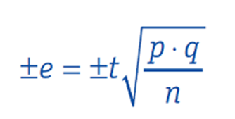
e = sampling error, i.e. the fluctuation range (±) in per cent around the measured sample value within which the „true“ value (in the population) lies with a certain probability.
t = indicator for the specified certainty of the inference from the sample to the population (the choice of t determines the significance level).
The following table shows at which value of t the »true« value of the characteristic lies within the interval p ± e and with what probability.
| t-value | Confidence probability (significance level) (in %) |
|---|---|
| 1 | 68,3 |
| 1,96 | 95,0 |
| 2 | 95,5 |
| 3 | 99,7 |
| 3,29 | 99,9 |
p = proportion of people in the population who have a certain characteristic (e.g. proportion of users of brand X).
q = proportion of people in the population who do not have a certain characteristic (e.g. proportion of non-users of brand X).
The product p - q - and thus also the sampling error - is greatest for a given sample size if p has a value of 50. This most unfavourable value in relation to the sampling error is always assumed if p is not known.
n = sample size
The following example illustrates the calculation of the sampling error: With a sample size of n = 400 and the assumption that p = 50 per cent, the sampling error is ± 5 per cent if t = 2 is selected. Accordingly, the „true“ value of p, i.e. the proportion of users of brand X in the population, is between 45 and 55 per cent with a probability of 95.5 per cent (t = 2) (cf. Ter Hofte-Fankhauser/Wälty, 2013, p. 50 f.) The calculated interval is also referred to as the confidence interval of the proportion value p. As the following figure shows, the size of the sampling error at a given significance level depends on the size of the sample on the one hand and on the value p on the other.
| Sample size n | P q | 50 50 | 45 55 | 40 60 | 35 65 | 30 70 | 25 75 | 20 80 | ... ... |
|---|---|---|---|---|---|---|---|---|---|
| ... | ... | ... | ... | ... | ... | ... | ... | ... | |
| 100 | 10,0 | 9,9 | 9,8 | 9,5 | 9,2 | 8,7 | 8,0 | ... | |
| 200 | 7,1 | 7,0 | 6,9 | 6,7 | 6,5 | 6,1 | 5,7 | ... | |
| 300 | 5,8 | 5,7 | 5,7 | 5,5 | 5,3 | 5,0 | 4,6 | ... | |
| 400 | 5,0 | 5,0 | 4,9 | 4,8 | 4,6 | 4,3 | 4,0 | ... | |
| 500 | 4,5 | 4,4 | 4,4 | 4,3 | 4,1 | 3,9 | 3,6 | ... | |
| 600 | 4,1 | 4,1 | 4,0 | 3,9 | 3,7 | 3,5 | 3,3 | ... | |
| 700 | 3,8 | 3,8 | 3,7 | 3,6 | 3,5 | 3,3 | 3,0 | ... | |
| 800 | 3,5 | 3,5 | 3,5 | 3,4 | 3,2 | 3,1 | 2,8 | ... | |
| 900 | 3,3 | 3,3 | 3,3 | 3,2 | 3,1 | 2,9 | 2,7 | ... | |
| 1000 | 3,2 | 3,1 | 3,1 | 3,0 | 2,9 | 2,7 | 2,5 | ... | |
| ... | ... | ... | ... | ... | ... | ... | ... | ... | ... |
Strictly speaking, the calculation of the sampling error and the confidence interval is only permitted if the following condition is met: n - p - q ≥ 9 (Bortz/Schuster 2010, p. 104 f.). This is the case in this example, as the following applies: 400 - 0.5 - 0.5 = 100. The sampling error can be calculated not only for percentage distributions, but also for sample averages of metric data (Homburg, 2015, p. 323 ff.).

Additional material for the individual chapters:
3-2: Telecoms advertising - importance of mirror neurons for emotional reactions
3-4: Measuring implicit attitudes using the implicit association test (IAT)
3-6: Subjective perception: Are two tables identical or not?
3-7: The eye eats too: Visual perception influences our feeling of hunger
3-8: Febreze: Importance of habitualised decisions for marketing
4-2: Operationalisation and measurement of the environmental orientation of EU citizens
4-5: Screening questionnaire for the realisation of a predefined sample
4-6: Conception of an interview guide for a qualitative survey
4-7: Observation of individual eating behaviour in the „restaurant of the future“
4-8: Product positioning: Positioning a smartphone brand in the competitive environment
4-9: Testing the preference effect of smoothie properties using choice-based conjoint analysis
7-1: Kindle Fire - Influencing the perception of net benefit through advertising
7-2: Determining the optimal electricity tariff using choice-based conjoint analysis
7-4: Influencing perceived price favourability through umbrella pricing
7-7: High attractiveness of private financing and leasing offers for cars
8-1: Product positioning: Code analysis of the brand presence of two sparkling wine brands
8-12: Advertising impact analysis of digital communication tools
8-3: The power of megatrends and the future of safety and quality
8-5: Guerrilla communication: using a neo-Nazi march for a good cause
8-7: Integrated communication using the example of the Hypoxi brand
You are currently viewing a placeholder content from Instagram. To access the actual content, click the button below. Please note that doing so will share data with third-party providers.
More InformationYou are currently viewing a placeholder content from YouTube. To access the actual content, click the button below. Please note that doing so will share data with third-party providers.
More Information


Study Service Centre
+49 3631 420-222
House 18, Level 1, Room 18.0105